Viewing Array Statistics and Data

After you add an array to the Array View, you can examine array statistics and view array data by selecting the view you want from the provided view dropdown.

The default view is Statistics.

To get started examining array statistics and data, see Adding Arrays to the Array View.

In the Array View, you can also access the Configuration Options dialog, from which you can:

Cast an array to a different type.
Isolate and view a smaller portion of data by either slicing the array or adding a stride.
Specify an array filter.

For more information on using the Configuration Options dialog, see Configuring Arrays.

On this page:

Viewing Array Statistics

The Statistics view provides access to statistical information generated from the array values.

Figure 64. The Array Statistics view

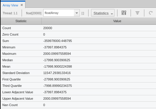
The above is a one-dimensional floating point array composed of 20,000 elements, identified under the Count statistic. See Array Statistics Detail in the following section for information on all displayed statistics.

Array statistics are also available through the CLI, as switches to the dprint command.

Array Statistics Detail

If you have added a slice (see Slicing Arrays), these statistics describe only the information currently being displayed; they do not describe the entire array. For example, if an array includes positive values, but a slice omits array values that are more than 0, the median value is negative even though the entire array’s real median value is more than 0.

Count: The total number of displayed array values. If you’re displaying a floating-point array, this number doesn’t include NaN or Infinity values.
Zero Count: The number of elements whose value is 0.
Sum: The sum of all the displayed array’s values.
Minimum: The smallest array value.
Maximum: The largest array value.
Median: The middle value. Half of the array’s values are less than the median, and half are greater than the median.
Mean: The average value of array elements.
Standard Deviation: The standard deviation for the array’s values.
Quartiles, First and Third: Either the 25th or 75th percentile values. The first quartile value means that 25% of the array’s values are less than this value and 75% are greater than this value. In contrast, the third quartile value means that 75% of the array’s values are less than this value and 25% are greater.
Lower Adjacent Value: This value provides an estimate of the lower limit of the distribution. Values below this limit are called outliers. The lower adjacent value is the first quartile value minus the value of 1.5 times the difference between the first and third quartiles.
Upper Adjacent Value: This value provides an estimate of the upper limit of the distribution. Values above this limit are called outliers. The upper adjacent value is the third quartile value plus the value of 1.5 times the difference between the first and third quartiles.
Denormalized Count: A count of the number of denormalized values found in a floating-point array. This includes both negative and positive denormalized values as defined in the IEEE floating-point standard. Unlike other floating-point statistics, these elements participate in the statistical calculations.
Infinity Count: A count of the number of infinity values found in a floating-point array. This includes both negative and positive infinity as defined in the IEEE floating-point standard. These elements do not participate in statistical calculations.
NaN Count: A count of the number of NaN (not a number) values found in a floating-point array. This includes both signaling and quiet NaNs as defined in the IEEE floating-point standard. These elements do not participate in statistical calculations.
Checksum: A checksum value for the array elements.

Viewing Array Data

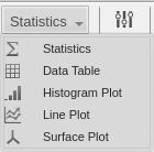
To view your data, select either Data Table, Histogram Plot, Line Plot, or Surface Plot from the view dropdown.

Different datasets can require different views to display their data. For example, you can use a histogram plot to see the distribution of a dataset, or line and surface plots to view trends or slope.

The examples that follow display all the data for an array. To display a subset, you can slice the data. See Slicing Arrays.

Data Table View

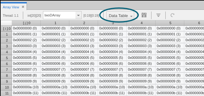
The Data Table view shows two dimensions of array data for the array expression that you have added to the Array View.

Figure 65. Array View > Data Table view

Configure the Data Table Array Dimensions

Click on the Array View toolbar to open the Configuration Options dialog, where you can specify which dimensions of the array are displayed as a row or a column by using the Dimension dropdown controls in the Slice table.

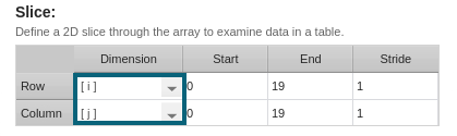
For more information about using the Configuration Options dialog to add slices and strides for the array, see Adding a Slice and Stride to the Data Table View.

Configure the Data Table Data Format

Click on the Array View toolbar to open the Configuration Options dialog, where you can specify how to format the data in the Data Table.

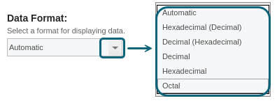
After you select a format for displaying the data, you can:

Click Apply to view your changes immediately in the Data Table view; the dialog box remains open so you change your selection.
Click OK to apply and save your changes; the dialog box closes automatically.
Click Reset to cancel your changes; the dialog box resets to the Data Table's original format setting, and you can then click Apply to re-set the Data Table view to this default format.

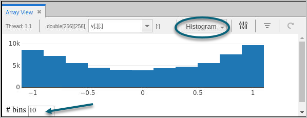
Histogram Plot View

By default, the Histogram Plot view displays 10 bins, or buckets.

Figure 66. Array View > Histogram plot with the default number of bins

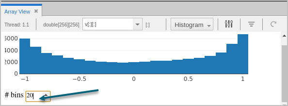
You can change the number of bins to evaluate a different dataset distribution.

Figure 67. Array View > Histogram plot with a modified number of bins

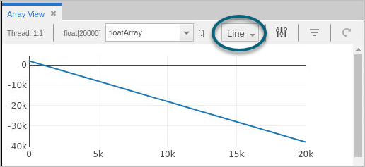
Line Plot View

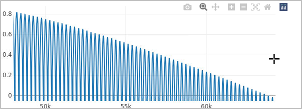
To display your data as x and y coordinate pairs, use the Line Plot view. This view is useful to plot trend lines in your one-dimensional datasets, as shown in Figure 68.

Figure 68. Array View > Line plot one-dimensional dataset

For higher-dimensional datasets in the Array View, the Line Plot view displays a flattened, one-dimensional dataset. For example, given an array like this:

[[31 12 43][42 1 16][0 42 0]]

The Line Plot displays a flattened array, like so:

[31 12 43 42 1 16 0 42 0]

Surface Plot View

The Surface Plot view displays two-dimensional datasets as a surface in two or three dimensions. The dataset’s array indices map to the first two dimensions (X and Y axes) of the display, and the values map to the height (Z axis). This can be useful to show a relationship across three variables and to observe trends in two-dimensional datasets.

The Surface Plot view is supported only on Linux-x86-64, Linux ARM64, and macOS and requires OpenGL version 2.1 or later.

Figure 69. Array View > Surface plot

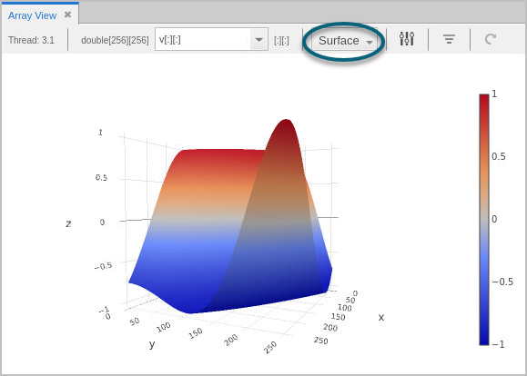
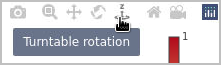
Use the plot controls to rotate or zoom the display, or to download an image of the display.

Updating the View

After advancing your program, the view does not update automatically. To refresh the display, click the update button ().

Changing the Thread of Focus

If you change the program’s thread of focus, it’s not reflected in the array displayed in the Array View, which displays the original thread of focus when the array was added to the view. You can, however, maintain multiple arrays in the Array View that are tied to different threads of focus.

Zooming Into Data

To view some data in detail, use the zoom toolbar, which displays when you place your cursor inside the graph.

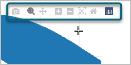
To zoom in, use one of the following methods:

Click .
Click and drag an area that you want to zoom in on.

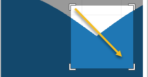
This results in TotalView zooming in on your data.

Figure 70. Array View > zooming in on data

To undo the zoom, use one of the following methods:

Double-click the graph.
Click .
Click .

If you know the indices you want to examine, you can also slice the array to view a subsection; see Slicing Arrays.